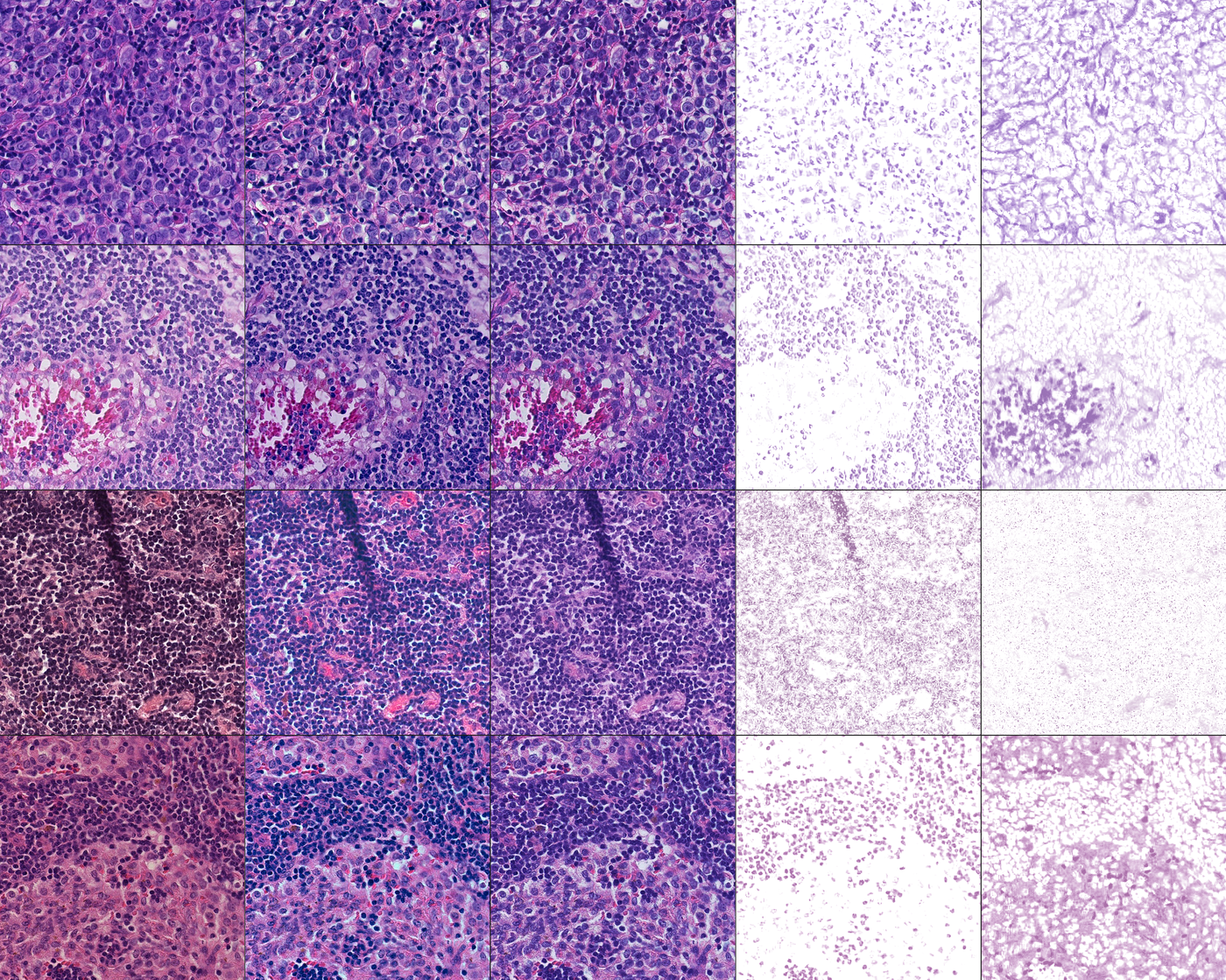
When tissue sections cut from the same paraffin block are sent to 66 different laboratories for routine H&E staining, the results look like they came from 66 different patients. A recent paper by Khan et al. (2026, Scientific Reports) demonstrated this by distributing serial sections of colon, kidney, and skin tissue to labs across 11 countries, scanning everything on the same scanner, and plotting the ratio of red to blue channel intensities. The spread was enormous — samples that should look near-identical deviated wildly from a balanced 1:1 colour ratio.
This is probably unsurprising to people that work with multiple datasets of histopathology WSIs, but I personally thought that these results were wild. For such a standardised diagnostic practice, it is a little bit insane that there can be so much variability.
This variability is pretty important to consider for downstream tasks in WSI analysis – these color shifts are going to affect any deep learning model you use, and they also affect the way pathologists themselves interpret the slides. Khan et al. showed this directly by running the same nucleus segmentation model (Cellpose-SAM) with identical hyperparameters across the 66 differently-stained versions of the same colon tissue: it produced nucleus counts ranging from under 10,000 to over 100,000. Same tissue content, same model, same parameters, wildly different results. The problem compounds when you try to deploy AI tools across institutions. A model trained on data from one centre’s staining profile will encounter a distribution shift when applied to slides from another centre, and this shift has nothing to do with biology (and distribution shift is definitely a well recorded phenomenon in terms of deployment of digital pathology systems).
This is the problem that stain normalisation (computationally transforming images so they appear as though they were stained by the same protocol) tries to mitigate. Stain deconvolution, a related technique, goes further by separating the contributions of individual stains. Both are widely used, but the mathematical details of how they work (and where they break down) are interesting to examine, especially if you’re as nerdy as I am.
How H&E staining produces color
Hematoxylin is a basic (cationic) dye. It binds to acidic cellular structures — primarily the phosphate groups in DNA and RNA — which is why cell nuclei appear blue-purple in a well-stained section. Eosin is acidic (anionic) and binds to positively charged structures such as cytoplasmic proteins and collagen, producing the characteristic pink-red of cytoplasm and extracellular matrix.
When white light passes through a stained tissue section, each stain absorbs certain wavelengths according to its absorption spectrum. The light that reaches the camera sensor is whatever wasn’t absorbed. The colour you see in the digital image is therefore a function of how much of each stain is present at that location and what each stain’s spectral absorption profile looks like.
The physics of this absorption follows Beer-Lambert’s law: the transmitted light intensity at a given wavelength decreases exponentially with the concentration of the absorbing substance and the path length through the tissue. This exponential relationship is the crux of the mathematical problem — in raw RGB pixel space, the contributions of hematoxylin and eosin are tangled together multiplicatively, which makes them difficult to separate.
Optical Density helps us solve this problem
The trick is to convert from transmitted light intensity to optical density (OD) by taking the negative logarithm:
where I is the measured intensity and I₀ is the intensity of the illumination source (typically estimated from the brightest region of the slide, i.e., the background glass).
Why does this help? Because of how logarithms interact with multiplication. If two stains contribute multiplicatively to the transmitted intensity (as Beer-Lambert tells us they do), taking the log converts that product into a sum. In optical density space, the total absorbance at each pixel is the sum of contributions from each stain. This additive relationship is what makes linear algebra applicable.

We can now write the optical density at each pixel as a matrix equation:
Here, OD(λ) is a 3×1 vector (one optical density value per RGB channel), S is a 3×2 matrix whose columns are the stain basis vectors — the characteristic optical density profile of hematoxylin and eosin at each of the three RGB wavelengths — and c is a 2×1 vector of stain concentrations at that pixel.
The stain basis vectors encode the “colour signature” of each stain. Pure hematoxylin absorbs strongly in certain wavelength bands; pure eosin absorbs in others. The concentration vector tells you how much of each stain is present. If you know S, you can solve for c by computing the pseudo-inverse of S and multiplying: c = S⁺ · OD. This gives you separate concentration maps for hematoxylin and eosin — that is stain deconvolution.
For stain normalisation, the idea extends naturally. If you deconvolve a source image to get its concentrations c_source, and you have a target stain matrix S_target from a reference image, you can reconstruct a normalised image by combining S_target · c_source. You keep the tissue’s structural information (encoded in the concentrations) but swap the colour appearance to match the reference.
The entire approach hinges on estimating the stain matrix S accurately. The two most widely used methods for doing this — Macenko and Vahadane — take different approaches.
Macenko: SVD in optical density space

Macenko’s method (2009) estimates the stain matrix using singular value decomposition (SVD). The intuition is geometric. If you plot the optical density values of every tissue pixel in 3D RGB-OD space, the points will cluster along a roughly planar region, because most of the variance in H&E images comes from just two (assumed) sources of absorption. SVD identifies this plane by finding the two directions of greatest variance.
The algorithm works as follows. First, convert all tissue pixels to optical density and discard background pixels (those below an OD threshold). Apply SVD to the resulting matrix of OD values. The first two singular vectors define the plane of maximum variance. Project all OD pixels onto this plane, reducing the problem to two dimensions.
Within this 2D projection, the algorithm identifies the two stain vectors as the directions corresponding to extreme angular positions — typically the 1st and 99th percentiles of the angular distribution of projected points. The reasoning is that pixels dominated by hematoxylin will cluster at one angular extreme, and pixels dominated by eosin at the other. The two resulting direction vectors, mapped back to 3D OD space, become the columns of the stain matrix S.
For normalisation, you estimate S_source from your input image and S_target from your reference image, deconvolve the source using S_source, optionally rescale the concentration histograms, and reconstruct with S_target.
The method is fast (SVD is a closed-form computation) and works well when both stains are well-represented in the image. It struggles when one stain dominates heavily — for instance, in regions of dense stroma with little nuclear material — because the angular distribution becomes skewed and the percentile-based stain vector estimation can pick up noise. It also assumes the data genuinely spans a 2D plane, which may not hold if there are additional chromophores (e.g., brown DAB in immunohistochemistry) or significant imaging artefacts.
Vahadane: sparse non-negative matrix factorisation

Vahadane’s method (2016) tackles the same decomposition problem but uses sparse non-negative matrix factorisation (SNMF) instead of SVD. The problem is framed directly as: given the optical density matrix of the image, find a stain matrix S and concentration matrix C such that OD ≈ S · C, subject to the constraints that all entries of both S and C are non-negative.
The non-negativity constraint is physically motivated — optical density and stain concentrations cannot be negative. The sparsity constraint, applied to C, encourages each pixel to be explained primarily by one stain rather than a mixture. This is biologically reasonable: most nuclear pixels are predominantly hematoxylin, most cytoplasmic pixels are predominantly eosin.
The optimisation alternates between updating S (with C fixed) and updating C (with S fixed), iterating until convergence. This is computationally more expensive than Macenko’s one-shot SVD — the iterative optimisation can take longer, especially on large images.
The paper by Khan et al. found that Vahadane performed worst among all methods on colour transfer metrics across all three tissue types. The qualitative pathologist assessment confirmed this: Vahadane tended to wash the entire image pink, effectively discarding the hematoxylin component. This is a failure mode that can occur when the SNMF optimisation converges to a solution where nearly all signal is attributed to a single stain basis vector. The sparsity constraint, intended to improve separation, can instead collapse one channel when initialisation or convergence criteria aren’t well calibrated — especially when applied to morphologically homogeneous regions or whole-slide images where eosin-stained content vastly outweighs nuclear material.
Vahadane did, however, achieve the best structural similarity scores (SSIM ≥ 0.967 across all tissue types). SSIM is a perceptual metric that compares two images in terms of luminance, contrast, and structural patterns — it outputs a value between 0 and 1, where 1 means the images are identical. In this context, SSIM was computed between each method’s normalised output and the original unnormalised image, so a high score means the method didn’t alter the image’s spatial structure much. Vahadane’s high SSIM follows directly from its relatively conservative colour transformation: it preserves pixel-level structure, but seemingly at the cost of not actually normalising the stain appearance.
Reinhard: statistical colour transfer in lαβ space

Reinhard normalisation (2001) takes a completely different approach — it doesn’t attempt to understand stains at all. Instead, it performs statistical colour matching between source and reference images in the lαβ colour space.
A brief explanation of lαβ is probably warranted here. It’s a colour space derived from human perception studies, designed so that its three channels (l for luminance, α for a yellow-blue axis, β for a red-green axis) are approximately statistically independent of each other. In RGB, the three channels are highly correlated — a brighter pixel tends to be brighter in all three channels simultaneously. In lαβ, this correlation is largely removed, which means you can manipulate each channel independently without introducing unexpected colour shifts.
Reinhard normalisation converts both the source and reference images to lαβ, computes the mean and standard deviation of each channel for both images, standardises each source channel to zero mean and unit variance, and then rescales using the reference’s mean and standard deviation. The transformation is linear and global — the same shift and scale is applied to every pixel.
This simplicity is a strength for speed and reproducibility, but also a limitation. The method assumes the colour difference between source and reference can be captured by a per-channel linear transformation. For subtle staining differences, this often works well. For large shifts (heavily over- or under-stained slides), a linear correction may not be sufficient.

Histogram matching: brute-force distribution alignment

Histogram matching goes further than Reinhard by aligning the full colour distributions rather than just the first two moments. For each colour channel, the method computes the cumulative distribution function (CDF) of both source and reference, then finds the pixel value mapping that transforms the source CDF into the reference CDF. The transformation can be non-linear, which gives it more flexibility than Reinhard’s linear scaling.
Khan et al. found that histogram matching was the best-performing traditional method across all three tissue types on colour transfer metrics, achieving the highest intersection and PCC scores and the lowest Euclidean distance and JS divergence. On kidney tissue, the margin was large (PCC of 0.985 vs. 0.927 for the next best method). Histogram matching also achieved the best FID scores for skin and kidney, indicating that high-level perceptual features were well preserved.
Part of this strong performance likely comes from the study’s design itself, however. Because all sections originated from the same tissue block, the underlying tissue content distributions were similar across samples. When content is held roughly constant and only colour varies, directly aligning colour distributions is a well-matched strategy. In a more heterogeneous dataset — say, comparing a section rich in mucosa to one dominated by smooth muscle — histogram matching might overfit to content differences rather than staining differences.
An important methodological detail from the paper: the authors applied normalisation to whole tissue images at 10× magnification rather than patch-by-patch. They specifically note that this avoided tiling artefacts that can arise when patches are normalised independently. This is a practical consideration that’s easy to overlook — computing colour statistics globally and applying them globally produces more spatially consistent results than computing and applying them locally (somewhat obviously?).
GAN-based approaches
Khan et al. also evaluated CycleGAN (with both ResNet and UNet generators) and Pix2pix (with UNet and DenseUNet generators). CycleGAN learns unpaired image-to-image translation using cycle-consistency loss, meaning it doesn’t require pixel-aligned source-target pairs. Pix2pix requires paired data; the authors created this by pairing each reference tile with its grayscale version, training the model to map grayscale to the reference colour profile.
The GAN-based methods produced reasonable colour transfer and, in the foundation model feature analysis (UNI-2 + t-SNE), the CycleGAN variants yielded the most compact feature clusters — suggesting they produced the most internally consistent representations. But they also introduced hallucination artefacts. CycleGAN (ResNet) generated spurious structures in adipose tissue regions and tile-boundary artefacts at tissue compartment borders. Pix2pix (DenseUNet) altered the colour of some smooth-muscle nuclei from blue to red.
The authors attribute these problems partly to data scarcity — with only one WSI per lab, the models were far below the data volume needed for robust generalisation. GANs also add operational complexity: they require training (CycleGAN variants took up to several days on a single V100 GPU), and retraining may be needed when the target domain changes.
Things worth thinking about more carefully
Reference image selection is underspecified. The paper selected reference images computationally — the sample with the red-to-blue channel ratio closest to 1:1 for each tissue type. This is a reasonable heuristic, but the choice of reference fundamentally determines the normalisation output, and there’s no consensus on how to make this choice optimally. A reference that produces good results for one downstream task might be suboptimal for another. The paper’s qualitative evaluation illustrates this: histogram matching improved heavily over-stained images when normalising to the chosen reference, but pushed under-stained images too far toward pink. A different reference might reverse this pattern.
Patch-level vs. whole-slide normalisation matters more than people assume. Most computational pathology pipelines tile WSIs into patches for processing at 20× or 40×. When normalisation is applied per-patch, each tile’s colour statistics are computed independently, which means adjacent tiles with different tissue composition (say, one mostly stroma, one mostly epithelium) may be normalised differently. This can introduce spatial inconsistencies that weren’t present in the original image. The paper’s results — using whole-slide normalisation at 10× — suggest that computing statistics globally and applying them at the slide level produces more uniform results. When that’s computationally feasible, it’s worth considering.
Normalisation interacts with downstream tasks in non-trivial ways. The nucleus segmentation experiment in the paper is a case in point. The methods that scored best on colour transfer metrics (histogram matching, CycleGAN ResNet) didn’t uniformly produce the most accurate nucleus counts. And the foundation model feature extraction experiment revealed something concerning: all normalisation methods substantially shifted the feature space representation relative to unnormalised images. If a foundation model trained on diverse data is still sensitive to normalisation choice, the assumption that large-scale pretraining confers stain invariance may need qualifying. At minimum, it’s worth checking whether your downstream model’s performance is robust to the specific normalisation method and reference image you’ve chosen.
Practical guidance depends on your specific situation. If your primary concern is colour consistency for a classification or detection model trained on data from a known centre, Reinhard or histogram matching are strong starting points — fast, training-free, and effective when tissue content is reasonably similar between source and target. If you need the separated stain channels themselves — for nuclear segmentation, stain quantification, or interpretability — Macenko or Vahadane give you deconvolved concentration maps, with Macenko being faster and Vahadane being more theoretically principled (though, as this paper shows, not always more effective in practice). If you have substantial training data and computational resources, GAN-based methods can learn more complex transformations, but you should inspect outputs carefully for hallucination artefacts — especially at tissue boundaries and in regions with unusual morphology.
The broader takeaway from Khan et al.’s dataset is that inter-laboratory staining variation is large — much larger than the datasets typically used for benchmarking can capture. Any normalisation strategy needs to be evaluated against a range of staining conditions, because methods that work well for moderate colour shifts can fail on the extremes, and vice versa. The dataset itself (available as open access) is a useful resource for anyone developing or evaluating normalisation pipelines, precisely because it isolates staining variation from tissue content variation in a way that smaller studies cannot.
Leave a Reply