Burhan Anis

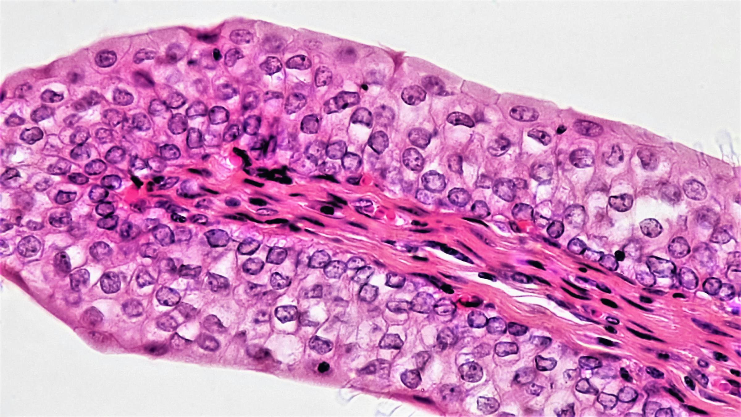
This article describes my development of a fully-supervised deep learning model to detect cancer metastases in histopathological whole slide images. I’ve written it in a format that should allow someone who knows a little about data science to be able to implement this themselves alongside my own Github repository. The aim of the article is to introduce histopathology as a medical imaging modality and how deep learning can be used for some basic classification tasks. You can download the data (the CAMELYON16 Dataset) from this link. I recommend using AWS S3 to do so.

What is Histopathology?

Histopathology, simply put, is the examination of tissue at a microscopic level, with the goal of identifying and describing how disease presents itself. In my PhD, I focus on lymph nodes (LNs), which act as filters within the lymphatic system and play a key role in immune function. Specifically, my work examines cases where cancer originating elsewhere in the body has spread to these lymph nodes, a process known as lymph node metastasis.

Histological samples are first collected from the body via surgery or biopsy (or autopsy). Once tissue has been collected for histopathological examination, it must first be prepared so that it can be viewed under a microscope. This tissue is preserved, processed, and cut into extremely thin sections, which are placed onto glass slides. To make the different structures within the tissue visible, the slides are commonly stained using haematoxylin and eosin (H&E), the standard stain in histopathology (though there are other stains as well). Haematoxylin stains cell nuclei a blue–purple colour, while eosin stains the surrounding tissue and cytoplasm in shades of pink. Together, this staining highlights the overall tissue architecture and cellular detail, allowing pathologists to examine normal and abnormal features at a microscopic level.

Digital Pathology

Traditionally, histological slides were examined directly by pathologists using a light microscope, with diagnoses made by visually inspecting the stained tissue at different magnifications. While this approach is still widely used, advances in imaging technology have enabled the digitisation of histology slides, a field known as digital pathology. In this process, glass slides are scanned using specialised high-resolution scanners to produce detailed digital images that capture the entire tissue section (again, at different magnifications, more on this later). These digital slides can be viewed on a computer in much the same way as using a microscope, but with several added benefits. Digitisation allows slides to be stored, shared, and reviewed remotely, supports easier collaboration between clinicians and researchers, and, most importantly for us, enables the application of image analysis and artificial intelligence methods to assist with diagnosis and research.

Whole Slide Images

These digital images of pathology slides are known as whole slide images, or WSIs. These are not your typical PNG or JPEG image files, however. Because these slides are being digitised at multiple magnifications, some of which are very high (for example, 40×), there is a large amount of data to store within a single slide. To manage this, WSIs are saved in specialised formats (tif, tiff, svs, etc) that use a pyramidal structure, meaning the same image is stored at several resolutions within one file. This allows users to smoothly zoom in and out, similar to using a microscope, without needing to load the entire high-resolution image at once – but, this requires specialised software. The actual files are very large, and very unruly to work with in a computer vision workflow. For example, the CAMELYON17 dataset, a very well-known breast lymph node metastases dataset, approaches 3TB of data with just 1000 images.

WSI Classification

We will consider the task of binary classification – ie, given a lymph node histology slide, can we predict whether or not the slide contains cancer metastasis? We’ll achieve this goal using a Convolutional Neural Network (CNN), though I do hope to write a tutorial on how this can be done with newer models such as Transformers. Specifically, we will choose the ResNet50 CNN, which is very commonly used in medical imaging research and is easily implemented through PyTorch. We will be using an open-source dataset called the CAMELYON16 data set (CAncer MEtastases in LYmph nOdes challeNge 2016), which is a collection of histopathological samples from the breast.

Fully Vs Weakly Supervised Learning

The ResNet50 has a default image input size of 256×256 pixels. Since these images are so huge, and because fine cellular detail matters very much to this task, compression is not an option – but we have billions of pixels, so this seems to be a problem. The solution is that we don’t feed the whole slide into the network as a single input, but rather we tile the image up into patches of our desired input size – use these for training, and then at the inference stage, we can aggregate the patch level predictions into a slide level prediction.

In fact, the tiling up of our slides means there is two different paradigms of model we can use. The first is fully supervised learning, in which every patch has a label – ie, we have the regions of metastases in our training slides fully annotated (we know the coordinates of the polygon that bounds these regions), which means we know that if a patch extracted from within these boundaries that it is tumor, and anything else is negative. In a weakly supervised setting, our training slides only have one label per slide, ie, we know there is metastasis somewhere in the slide (or not), but we don’t know exact coordinates. In this case, the patch level labels are ambiguous and the model learns which patches are most discriminative.

These two different paradigms reflect a very important aspect of histological image processing. Using a fully supervised paradigm incurs a much higher burden upon the pathologists that have to carefully annotate these images, whereas weakly supervised datasets are much easier to annotate/datasets can be generated by matching pathology reports to images without the need for annotation at all. In the first year of my PhD, I did a systematic review and meta-analysis of ~80 papers looking at LN metastases detection in WSIs, and found that weakly supervised methods do not perform any worse, statistically, than fully supervised methods, and this explains why this paradigm has become the most dominant one over the last 10 years.

This being said, however, we will focus on the fully supervised paradigm, as the dataset we are using (CAMELYON) is fully annotated anyway.

WSI Pre-processing – Tissue Region Selection

Generating 256x256px tiles from images which can be hundreds of thousands to billions of pixels large will still leave us with many, many patches. Looking at some of the slides in the CAMELYON16 dataset, we see that there is actually lots of white-space in them (ie, non-tissue regions). Our first step will be to reduce data by creating a pipeline that will generate image patches from only the tissue regions.

An option for this is to throw another neural network at the problem – one trained to identify tissue pixels. This is inefficient and unnecessary, however. We observe that the pixel intensities are quite binary on these images – the tissue is blue/purple and the background is solid white. We can deploy classical computer vision techniques to accomplish the tissue segmentation task – namely Otsu’s Thresholding. We use the following steps:

• Each WSI is first opened at a low magnification level to provide a coarse representation of the tissue and background.
• This low-resolution image is converted from the standard RGB colour space into HSV (hue, saturation, value). The saturation channel is particularly useful because stained tissue has a higher saturation than the white background of the slide.
• Otsu’s thresholding method is applied to the saturation channel to automatically separate tissue from background, producing a binary tissue mask.
• The resulting mask is used to identify regions that contain sufficient tissue, ensuring that empty or mostly background areas are excluded from further processing.
• A grid of candidate patch locations is overlaid on the slide at the target magnification level, using the tissue mask to determine which locations should be kept.
• For each valid location, a fixed-size patch (for example, 256 × 256 pixels) is extracted from the original high-resolution slide.
• Each patch is assigned a label (such as normal or tumour) based on pre-existing annotations or index information.
• Finally, patches are saved either as individual image files organised by label, or packed into efficient database formats such as LMDB or HDF5 to enable fast loading during deep learning training.

Below is the code snippet I use to accomplish this in my pipeline. As you can see, this is very easy with openslide and openCV. This is why I use Python.

def get_tissue_mask(slide, level):

    thumbnail_dims = slide.level_dimensions[level]
    slide_thumbnail  = np.array(slide.read_region([0,0], level, thumbnail_dims))
    slide_hsv = cv2.cvtColor(slide_thumbnail, cv2.COLOR_RGB2HSV)
    val, mask_thumbnail = cv2.threshold(slide_hsv[:,:,1], 0, 255, cv2.THRESH_OTSU)
    mask_thumbnail = cv2.morphologyEx(mask_thumbnail, cv2.MORPH_CLOSE, np.ones((5, 5)))

    return mask_thumbnail

def get_tissue_mask(slide, level):

    thumbnail_dims = slide.level_dimensions[level]
    slide_thumbnail  = np.array(slide.read_region([0,0], level, thumbnail_dims))
    slide_hsv = cv2.cvtColor(slide_thumbnail, cv2.COLOR_RGB2HSV)
    val, mask_thumbnail = cv2.threshold(slide_hsv[:,:,1], 0, 255, cv2.THRESH_OTSU)
    mask_thumbnail = cv2.morphologyEx(mask_thumbnail, cv2.MORPH_CLOSE, np.ones((5, 5)))

    return mask_thumbnail

You can see the full pipeline in the github repo.

Saving Image Patches

Even after the thresholding step, we still have hundreds of thousands or even millions of patches. It’s not exactly possible to save these all to disk (especially when you work on shared HPC systems, as I do), so the information about the patch coordinates and their labels and what slides they come from are saved to a dictionary (which is then saved as a pkl file), which can then be used in the training pipeline to load patches on the fly (though in my work, I don’t actually load on the fly for speed reasons, more explanation below).

Here is a scheme of the saved index:

slide_index = {
  "tumour_001": {
    "slide_path": "/data/slides/tumour_001.tif",
    "label": "tumour",
    "annotation_path": "/data/annots/tumour_001.xml",
    "level": 4,
    "work_level": 7,
    "magnification": 10.0,
    "patches": [
        (1024, 2048, False),
        (1280, 2048, False),
        (1536, 2048, True),
        (1792, 2048, True),
        (2048, 2048, False),
    ],
    "visualisation_coords": [
        (4, 8, False),
        (5, 8, False),
        (6, 8, True),
        (7, 8, True),
        (8, 8, False),
    ]
  }
}

slide_index = {
  "tumour_001": {
    "slide_path": "/data/slides/tumour_001.tif",
    "label": "tumour",
    "annotation_path": "/data/annots/tumour_001.xml",
    "level": 4,
    "work_level": 7,
    "magnification": 10.0,
    "patches": [
        (1024, 2048, False),
        (1280, 2048, False),
        (1536, 2048, True),
        (1792, 2048, True),
        (2048, 2048, False),
    ],
    "visualisation_coords": [
        (4, 8, False),
        (5, 8, False),
        (6, 8, True),
        (7, 8, True),
        (8, 8, False),
    ]
  }
}

Data Exploration

It’s always worth exploring the characteristics of your dataset before you jump into setting up your model training, as this allows you to identify potential issues you should address in your training loop implementations.

One of the main things I’ll look at here is the distribution of our classes, ie, how many tumour and non-tumour patches do we extract once we’ve found all the tissue tiles.

Below is the class distribution of the CAMELYON16 dataset, for 256×256 patches extracted at 10x magnification:

Normal: ~83.2%

Tumour: ~16.8%

We have an approximate 5:1 class imbalance within our dataset, and this will be very important to think about when we train our model. Note this is for the WHOLE dataset (ie, before any dataset splitting).

Addressing Class Imbalance

Over the course of developing a fully-supervised classification model for this dataset, I tried and tested many different techniques to improve performance, and here I’ll outline the ones that were the most useful.

Dataset Splits: Patches are split into training, validation, and test sets with care taken to preserve class balance in the training and validation splits, while test data are separated at the slide level to avoid information leakage.

Augmentation of only the Positive (Tumour Class): Within the training set, tumour patches are deliberately oversampled by duplication and flagged for augmentation, ensuring that positive examples are seen more frequently during optimisation. These flagged patches undergo additional random augmentations, including flips and rotations, which are biologically valid due to the absence of a canonical orientation in histological images.

Loss Function: During training, focal loss is employed with class weights derived from the training distribution to reduce the dominance of the majority (normal) class and focus learning on under-represented and hard-to-classify tumour patches.

Hard Example Mining: The benefit of focal loss is further reinforced through online hard example mining (OHEM), which dynamically selects the most challenging negative examples in proportion to the number of positive patches in each batch, concentrating model capacity on informative decision boundaries rather than the abundant ‘easy’ negatives.

Fully Supervised Training Pipeline

You can find my full training script on the GitHub repository linked here.

Below is an overview of the training pipeline used to train a fully supervised histology classifier:

• Slide Index Loading: The precomputed slide index is loaded (as explained above), which links each patch to its slide of origin and its class label (normal or tumour).
• LMDB Construction: We use these indexes to build a Lightning Memory Mapped Database (LMDB).
• Key Generation and Labelling: Unique keys are generated for every patch stored in the LMDB database, and corresponding binary labels are assigned.
• Data Splitting: Patches are divided into training, validation, and test sets. Test patches are separated at the slide level, while the remaining data are split into training and validation sets with class balance preserved.
• Class Imbalance Handling: As we said above, there is huge class imbalance in this dataset—there are many, many more normal patches than there are tumour patches. To address class imbalance, tumour patches in the training set are duplicated and flagged for augmentation, creating multiple augmented versions of each positive example. Basic preprocessing (tensor conversion and normalisation) is applied to all patches, while additional random augmentations (flips and rotations) are applied only to flagged training patches—these augmentations are okay because histology slides do not have a canonical orientation.
• Data Loading: Custom dataset and data loader classes read image patches and labels directly from the LMDB database, enabling fast batch loading during training. This method was benchmarked against on-the-fly patch loading, as well as against a HDF5 dataset and a simple filesystem storage dataset (each patch saved as a PNG), and was found to be the fastest.
• Model Architecture: A convolutional neural network (ResNet-50) is initialised and adapted for binary classification by replacing the final layer. We use a pre-trained CNN (on ImageNet), as this empirically showed faster training convergence time without loss of performance (in my own experiments).
• Loss Function: Focal loss is used with class weights derived from the training data to focus learning on harder and under-represented examples.
• Optimisation Strategy: The model is trained using the Adam optimiser, with a learning rate scheduler that reduces the learning rate when validation loss plateaus.
• Hard Example Mining: During each training batch, online hard example mining (OHEM) selects the most difficult negative patches relative to the number of positive patches, concentrating learning on challenging cases.
• Checkpointing and Early Stopping: Model weights are saved at regular intervals and whenever validation performance improves, with early stopping triggered if no improvement is observed.
• Test Evaluation: The best-performing model is evaluated on the held-out test set to estimate generalisation performance.
• Slide-Level Aggregation: Patch-level predictions from the test set are grouped by slide to produce per-slide probability and prediction summaries, which are saved for downstream analysis.

Model Evaluation

There is a separate inference script in the repository which can be used to evaluate the model. There is also a jupyter notebook which loads the slide index we created during pre-processing and the predictions index saved during inference to generate the confusion matrices and metrics I discuss below.

Once the model is trained and predictions are generated on the test set, we can overlay those predictions on our test slides (patch-wise), creating some nice prediction heatmaps. Let’s look at some of those:

For the slides with metastases in the ground truth, we see (visually, anyway), that there is pretty good agreement with our predictions! The regions of metastases seem to line up quite well. However, on the non-tumour regions and on the slides without tumour at all, we do also see lots of spurious false positives, which might be a problem. Let’s put some numbers to these:

We’ve got an accuracy of 97% – which is great! Right? Not necessarily – remember that our dataset was heavily class imbalanced, which also holds true for the test set, so there are other metrics which we ought to consider, which are more appropriate for evaluating this particular task. These are sensitivity (the ability of the model to evaluate those samples WITH the disease) and specificity (the ability of the model to correctly identify those WITHOUT the disease). Ie, the ability to identify true positives vs true negatives.

Our results given the above confusion matrix are:

Sensitivity: 87.1%

Specificity: 97.9%

These are good, but we would ideally want sensitivity to be higher than this. In the cancer detection case, it’s much more preferable to trade specificity for sensitivity, as the consequences of missing a cancer diagnosis are more severe than a false positive (though there are many things to be said about why this may not be the case – particularly in cases where a false diagnosis leads to treatment which unnecessarily impacts the quality of a patient’s life, not to mention the emotional toll this would have).

Getting the opinion of experts

To deepen the evaluation of our model, I would argue that it is also very crucial to get the perspective of actual clinical experts – ie, histopathologists in this case. They will be able to notice patterns in our false positives and false negatives which may help you to improve your model, and ultimately, these are tools for them anyway, so best involve them!

For this reason, I built a web-based WSI viewer to allow my histopathology supervisors to be able to interact with the predictions of my model in a dynamic and interactive way. It’s no good just sending them pictures like the ones in this article, because they need to be able to zoom and pan in order to see, in detail, what is going on. You can find this viewer here, loaded with a few test slides from CAMELYON16 with their predictions.

One of the main bits of feedback my supervisor’s had for me was that the model is great at spotting large metastases, but not very helpful for the small ones (micrometastases and isolated tumour cells). For them, the tool isn’t helpful, because they don’t struggle with the big ones anyway, they want a tool to help them with the small ones. They were also able to spot that many of the spurious false positives are specific cell types, like fat cells, or capillaries.

It is important to state, though, that the detection of small metastases is a field-wide problem. See this paper, which tested multiple large pathology foundation models and found that even the best ones were pretty much rubbish with ITCs (at 20x magnification anyway). It’s necessary to use higher magnification for smaller metastases, but this creates its own problem in the sheer amount of data created (there are hundreds of thousands of patches 10x, but tens of millions as we reach 40x). This is the problem that my PhD will focus on going forward: small object detection in multi-gigapixel images.

If you want to follow my progress, please do subscribe here.